Semantic Search with Embedding Models: A Practical Tutorial
Build a production-grade semantic search with embedding models: data prep, indexing, similarity, hybrid retrieval, re-ranking, evaluation, and scaling.
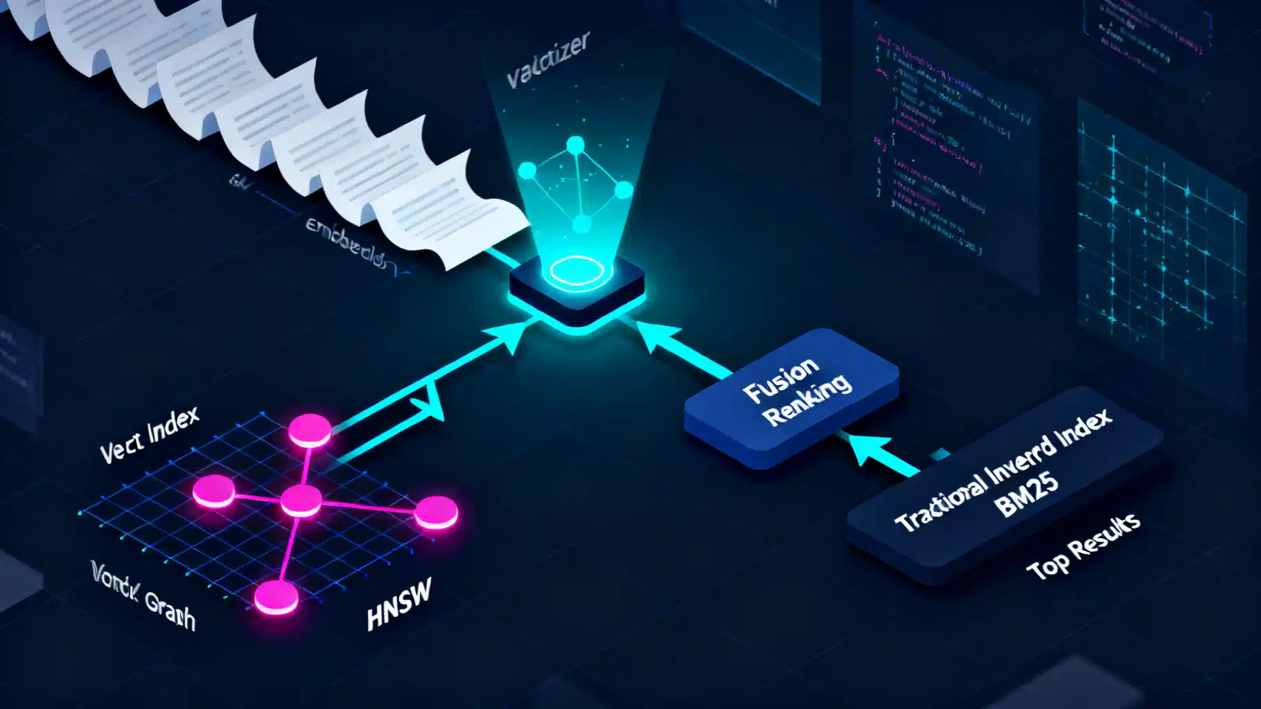
Image used for representation purposes only.
Overview
Semantic search replaces brittle keyword matching with meaning-aware retrieval. Instead of counting word overlaps, we embed queries and documents into a vector space where similar meanings are close together. In this tutorial, you will learn the core ideas behind embedding models, how to prepare data, build an index, choose similarity metrics, evaluate quality, and scale a system from prototype to production.
What you will build:
- A minimal semantic search pipeline using Python with FAISS
- A SQL-based variant using PostgreSQL with pgvector
- An end-to-end retrieval pipeline that supports hybrid (BM25 + embeddings) and re-ranking
By the end, you will understand not just how to implement semantic search, but also how to make pragmatic engineering decisions about models, indexing, evaluation, and operations.
How embeddings power semantic search
Embedding models map text to dense vectors, typically 256–1536 dimensions. Semantically related texts end up near each other, allowing nearest-neighbor search to retrieve relevant items even when exact keywords do not match.
Typical flow:
- Ingest content (documents, FAQs, product listings, tickets).
- Chunk content into passages (e.g., 200–400 tokens).
- Encode each passage into a vector and store alongside metadata.
- At query time, encode the user query, search the vector index for nearest neighbors, and return top-k passages.
- Optionally apply a cross-encoder re-ranker and assemble final answers.
Choosing an embedding model
Pick a model that matches your language, latency, and cost constraints. Common categories:
- Small, fast, general-purpose: all-MiniLM-L6-v2 (384d), e5-small, bge-small-en-v1.5
- Strong English retrieval: e5-base, bge-base-en-v1.5, mxbai-embed-large
- Multilingual: LaBSE, distiluse-base-multilingual, bge-m3, e5-multilingual
- Domain-tuned: models fine-tuned on finance, legal, or code
Guidelines:
- Start small for baseline latency and cost; upgrade only if quality demands it.
- Prefer models trained for retrieval tasks (contrastive learning with hard negatives).
- Use multilingual models if your corpus or users are cross-language.
- Keep vectors reasonably sized (384–768 dims) unless you truly need larger.
Data preparation and chunking
Chunking is as important as model choice.
- Split by semantic boundaries first (headings, paragraphs). Fall back to token-based splits.
- Typical chunk: 200–400 tokens with 20–40 token overlap to preserve context across boundaries.
- Store rich metadata: title, section, URL, timestamps, product IDs, language code, permissions.
- Normalize text: lowercase, trim whitespace, normalize unicode. Keep punctuation when helpful.
- Deduplicate aggressively (minhash or embedding-based clustering) to avoid repetitive results.
Example Python chunker using a sliding window:
import re

def simple_chunks(text, max_tokens=300, overlap=40):
    words = re.findall(r'\S+', text)
    i = 0
    chunks = []
    while i < len(words):
        chunk = words[i:i+max_tokens]
        chunks.append(' '.join(chunk))
        i += max_tokens - overlap
    return chunks
Quickstart: build a vector index with FAISS (Python)
This minimal example uses sentence-transformers and FAISS. It demonstrates ingestion, indexing, and search.
# pip install sentence-transformers faiss-cpu
from sentence_transformers import SentenceTransformer
import faiss
import numpy as np

# 1) Load an embedding model
model = SentenceTransformer('sentence-transformers/all-MiniLM-L6-v2')  # 384 dims

# 2) Example corpus
docs = [
    'How do I reset my password?',
    'Install the CLI with pip and authenticate using a token.',
    'Our warranty covers defects for two years from purchase.',
    'To deploy, run the docker compose file in the repo root.'
]

# 3) Encode and build index
emb = model.encode(docs, normalize_embeddings=True)  # shape: (n, 384)
index = faiss.IndexFlatIP(emb.shape[1])  # inner product with normalized vectors = cosine
index.add(emb.astype('float32'))

# 4) Query
query = 'I forgot my account credentials'
q_vec = model.encode([query], normalize_embeddings=True).astype('float32')
D, I = index.search(q_vec, k=3)

# 5) Show results
for rank, idx in enumerate(I[0], 1):
    print(rank, docs[idx])
Notes:
- When using cosine similarity with FAISS, normalize embeddings and use inner-product (IndexFlatIP) to emulate cosine.
- For larger corpora, switch to an approximate nearest neighbor (ANN) index such as HNSW or IVF-PQ.
Option B: PostgreSQL with pgvector
A relational database plus vectors is attractive for transactional workloads and RBAC.
Setup outline:
-- In Postgres with the pgvector extension installed
create extension if not exists vector;

create table passages (
  id bigserial primary key,
  doc_id text,
  content text not null,
  embedding vector(384),
  lang text,
  created_at timestamptz default now()
);

-- Index for cosine distance (use vector_l2_ops for L2)
create index on passages using ivfflat (embedding vector_cosine_ops) with (lists = 100);
Ingest from Python:
import psycopg2, numpy as np
from sentence_transformers import SentenceTransformer

model = SentenceTransformer('sentence-transformers/all-MiniLM-L6-v2')
conn = psycopg2.connect('dbname=demo user=demo password=demo host=localhost')
cur = conn.cursor()

texts = ['example one', 'example two']
vecs = model.encode(texts, normalize_embeddings=True)

for t, v in zip(texts, vecs):
    cur.execute('insert into passages (doc_id, content, embedding, lang) values (%s, %s, %s, %s)',
                ('d1', t, list(v), 'en'))
conn.commit()
Query with cosine distance (smaller is closer):
select id, content, 1 - (embedding <#> to_vector) as score
from passages, (select '[0.1,0.2,...]'::vector as to_vector) q
order by embedding <#> to_vector
limit 5;
Tip: For performance, set ivfflat lists roughly to sqrt(n_rows), and analyze the table after bulk loads.
Similarity metrics and normalization
- Cosine similarity: angle between vectors; robust across varying magnitudes. Normalize vectors to unit length. Works well for most embedding models.
- Inner product: proportional to cosine when vectors are normalized.
- Euclidean (L2): sometimes used; can underperform for some embedding models.
Rule of thumb: if the model was trained with cosine/contrastive losses, use cosine (or IP + normalization). Always confirm by A/B testing.
ANN index choices in practice
As your corpus grows, exact search becomes slow. ANN structures trade tiny recall loss for big speed gains.
- HNSW: excellent recall at low latency; memory-heavy. Great default up to tens of millions of vectors.
- IVF-Flat: partitions vectors into Voronoi cells (coarse quantizer), then searches a subset of lists. Good fit for disks and batching.
- IVF-PQ: adds product quantization to reduce memory; introduces quantization error; pair with re-ranking using originals if possible.
- DiskANN/SSG/NSG variants: advanced graph-based methods optimized for SSD.
Tuning knobs:
- HNSW: ef_construction (build accuracy), M (graph degree), ef_search (query recall/latency).
- IVF: nlist (number of clusters), nprobe (clusters probed per query).
- PQ: m (subquantizers), bits per code; trade accuracy for memory.
Strategy: pick HNSW for speed and simplicity; use IVF-PQ when memory is your bottleneck; always re-rank a larger candidate set with exact similarity.
Retrieval pipelines: hybrid and re-ranking
A strong production system rarely relies on a single signal.
- Hybrid retrieval: combine BM25 (lexical) with embeddings (semantic). This restores precision on rare or exact terms and maintains recall for paraphrases.
- Score fusion: normalize scores and combine (e.g., weighted sum), or use Reciprocal Rank Fusion (RRF) when score scales differ.
- Cross-encoder re-ranking: a bi-encoder (embedding) retrieves top-100; a cross-encoder then scores each candidate with full attention over query and passage. This boosts precision@k noticeably, with modest latency overhead.
Pseudocode for RRF:
# ranks_bm25 and ranks_vec are dicts: doc_id -> rank (1-based)
from collections import defaultdict

def rrf(ranks_bm25, ranks_vec, k=60):
    scores = defaultdict(float)
    for doc_id, r in ranks_bm25.items():
        scores[doc_id] += 1.0 / (k + r)
    for doc_id, r in ranks_vec.items():
        scores[doc_id] += 1.0 / (k + r)
    return sorted(scores.items(), key=lambda x: x[1], reverse=True)
Evaluating quality
Define a clear, reproducible evaluation loop.
- Metrics: Recall@k, Precision@k, MRR, nDCG@k. For QA: answer exact match or F1. For chat-augmented retrieval (RAG), judge answer helpfulness with human labels or LLM-assisted evaluation—validate with spot checks.
- Datasets: Create query–passage pairs from real logs. Mine hard negatives by retrieving with BM25 for embedding-trained models and vice versa.
- Protocol: Freeze a test split and run the same metrics for each change (model, chunking, index params). Track confidence intervals via bootstrapping.
Example evaluation snippet:
# qrels: dict query_id -> set of relevant doc_ids
# runs: dict query_id -> list of (doc_id, score) sorted desc

def recall_at_k(qrels, runs, k=10):
    hits, total = 0, 0
    for qid, rels in qrels.items():
        total += 1
        topk = [d for d, _ in runs.get(qid, [])[:k]]
        if any(d in rels for d in topk):
            hits += 1
    return hits / max(total, 1)
Target baselines:
- Good general-purpose retrieval on clean corpora: Recall@10 in the 0.85–0.95 range with hybrid + re-ranking.
- If you are below 0.75, examine chunking, model choice, and index recall.
Latency, memory, and cost planning
- Memory estimate: float32 uses 4 bytes per dimension. A 384d float32 vector is ~1.5 KB; 100M passages would be ~150 GB for raw vectors before index overhead. Using float16 halves memory with small accuracy loss.
- Latency budget: aim for p95 under 150 ms for retrieval-only; under 300 ms including re-ranking on 100 candidates. Parallelize and cache query embeddings.
- Batch offline encoding to amortize model costs. For fast online queries, keep the encoder on GPU or use a small CPU-friendly model.
Multilingual and cross-lingual retrieval
- Use a multilingual bi-encoder (e.g., bge-m3 or e5-multilingual) so that a query in language A can retrieve a passage in language B.
- Store a language code in metadata and prefer same-language results first; fall back to cross-lingual when needed.
- Tokenization and normalization vary by script; ensure proper unicode handling and stopword removal only if your lexical branch needs it.
Domain adaptation and fine-tuning
If off-the-shelf quality stalls:
- Hard-negative mining: retrieve top-k with the current system; label non-relevant high-scoring passages as negatives; continue contrastive fine-tuning.
- Instruction tuning: include task-specific prompts for queries and passages if your model supports it.
- Distillation: teach a smaller model to mimic a larger one’s similarity behavior for latency gains.
Security and privacy
- Redact PII before indexing when possible; store original text separately with stricter access.
- Encrypt in transit and at rest; use column-level encryption for sensitive fields.
- Enforce row-level security for multi-tenant systems; filter by tenant_id at query time.
- Respect right-to-erasure: maintain a deletion log and reindex or tombstone affected chunks quickly.
Observability and online quality control
- Log query embeddings, top-k doc IDs, and scores with anonymized query text.
- Track drift: monitor embedding vector norms, mean query length, and language mix.
- Add feedback loops: click signals, thumbs-up/down, and editorial labels. Use them to periodically refresh fine-tuning.
Troubleshooting checklist
- Irrelevant results? Verify you used the same model for indexing and querying and that vectors are normalized for cosine/IP.
- Missing rare terms? Add BM25 to your pipeline or upweight exact-entity matches.
- Duplicates in results? Deduplicate by doc_id or use maximal marginal relevance (MMR) during selection.
- Slow queries at scale? Switch to HNSW or IVF and re-rank a larger candidate pool; ensure indexes fit in RAM or use SSD-optimized engines.
- Mixed languages? Use a multilingual model and language-aware ranking rules.
Minimal end-to-end pipeline (Python)
# pip install sentence-transformers faiss-cpu rank-bm25
from sentence_transformers import SentenceTransformer
from rank_bm25 import BM25Okapi
import faiss, numpy as np

corpus = [
  'Reset your password via account settings or the reset email link.',
  'Install the CLI using pip install mycli and run mycli auth login.',
  'Warranty covers manufacturing defects for 24 months.'
]

# 1) Build BM25
bm25 = BM25Okapi([c.split() for c in corpus])

# 2) Build embeddings index
model = SentenceTransformer('sentence-transformers/all-MiniLM-L6-v2')
vecs = model.encode(corpus, normalize_embeddings=True).astype('float32')
index = faiss.IndexHNSWFlat(vecs.shape[1], 32)
index.hnsw.efConstruction = 80
index.add(vecs)

# 3) Query
query = 'I forgot my password'
q_vec = model.encode([query], normalize_embeddings=True).astype('float32')
D, I = index.search(q_vec, 5)

# 4) Hybrid RRF
bm25_scores = bm25.get_scores(query.split())
bm25_ranks = {i: rank+1 for rank, i in enumerate(np.argsort(-bm25_scores))}
vec_ranks = {int(i): rank+1 for rank, i in enumerate(I[0])}

def rrf(ranks_a, ranks_b, k=60):
    import collections
    s = collections.defaultdict(float)
    for d, r in ranks_a.items(): s[d] += 1.0/(k+r)
    for d, r in ranks_b.items(): s[d] += 1.0/(k+r)
    return sorted(s.items(), key=lambda x: x[1], reverse=True)

final = rrf(bm25_ranks, vec_ranks)
print([corpus[i] for (i, _) in final[:3]])
Production tips
- Cache query embeddings for frequent queries and use CDN for static search pages.
- Use background workers for re-indexing; keep a blue-green index to swap atomically on deploy.
- Version everything: model name, preprocessing steps, index parameters. Store them in the index metadata.
- For large organizations, wrap retrieval in a feature flag to safely A/B test new models.
Summary
Semantic search with embedding models delivers robust retrieval that understands meaning. Start with a small, strong bi-encoder, clean chunking, cosine similarity, and an HNSW or IVF index. Layer on hybrid BM25 and cross-encoder re-ranking to maximize precision. Measure with Recall@k and nDCG, iterate with hard negatives, and plan for security, observability, and operational excellence.
Armed with the patterns and snippets above, you can ship a reliable semantic search system and grow it confidently as your corpus and traffic scale.
Related Posts

Advanced Chunking Strategies for Retrieval‑Augmented Generation
A practical guide to advanced chunking in RAG: semantic and structure-aware methods, parent–child indexing, query-driven expansion, and evaluation tips.

React Drag and Drop Tutorial with dnd-kit: From Basics to Kanban
A hands-on React drag-and-drop tutorial using dnd-kit: from basics to a Kanban board, with accessibility, performance tips, and common pitfalls.