
Retrieval Pipeline Optimization Techniques: A Practical Playbook for Search and RAG
A practical playbook to optimize retrieval pipelines for search and RAG: metrics, chunking, hybrid retrieval, ANN tuning, re-ranking, and efficiency.
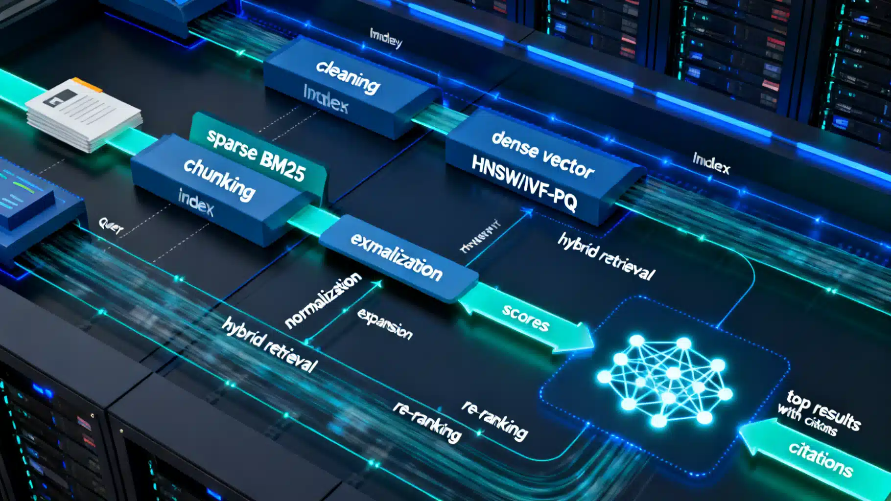
Image used for representation purposes only.
Overview
Retrieval is the backbone of both classic search engines and modern Retrieval-Augmented Generation (RAG) systems. A well-optimized retrieval pipeline finds the right passages quickly, cheaply, and reliably—so downstream rankers or LLMs can focus on reasoning rather than rummaging. This article is a practical playbook of techniques to boost quality (recall/precision), slash latency and cost, and harden your pipeline in production.
The Retrieval Pipeline, Decomposed
A typical production pipeline has these stages:
- Ingestion and preprocessing: clean, split, enrich, and deduplicate documents.
- Index building: sparse (BM25), dense (vector), or hybrid; set index parameters.
- Query processing: normalization, expansion/rewriting, intent detection, routing.
- First-stage retrieval: fast recall over millions to billions of chunks.
- Re-ranking: cross-encoder or LLM-based reranker for precision.
- Post-processing: diversification, deduping, safety/guardrails.
- Observability: logging, metrics, offline/online evaluation loops.
Think in stages because most optimizations are local and composable.
North-Star Metrics and Diagnostics
Define success with both offline and online signals.
Quality
- Recall@k: probability the gold document is in the top k retriever results (e.g., k=20).
- Precision@k: fraction of top-k that are relevant.
- nDCG@k or MRR: position-sensitive metrics that reward early hits.
- Coverage: fraction of queries that return at least one relevant result after filtering.
System
- Latency: p50/p95 per stage and end-to-end. Track CPU vs GPU time.
- Throughput/QPS: sustained and burst.
- Cost: $/1k queries, memory footprint, index build time.
- Stability: error rate, timeouts, tail latency volatility.
Always keep a query log and a labeled evaluation set that mirrors production distribution; update the set as content and behavior drift.
Corpus Preparation: Where Wins Start
- Cleaning and normalization: strip boilerplate, HTML, and scripts; normalize Unicode; collapse whitespace.
- Deduplication: near-duplicate detection with MinHash or SimHash; eliminate redundant chunks to reduce noise and cost.
- Chunking strategy: choose chunk size to balance context and specificity.
- Token-based: 200–400 tokens is a strong default for RAG; overlap 10–20% to preserve context boundaries.
- Semantic splits: split by headings/sections; use sentence boundaries to avoid mid-thought cuts.
- Adaptive chunking: shorter for dense, technical facts; longer for narrative/overview docs.
- Metadata enrichment: titles, headings, timestamps, authors, entities, language, access level. Good metadata enables precise filtering and boosts ranking.
- Fielded representation: store separate fields (title, body, abstract, code) to allow field-aware retrieval and boosts.
Indexing Strategies and Tuning
Choose the index by scale, latency targets, and content type.
Sparse (lexical)
- BM25 (or variants) excels on exact matches, names, and rare terms.
- Tune: stopword lists, stemming/lemmatization, per-field boosts (e.g., title x2–x5), and BM25 parameters k1/b.
- Add synonyms/aliases and controlled vocabularies for domain terms.
Dense (vector)
- Bi-encoder embeddings enable semantic matches, paraphrases, and recall on long-tail queries.
- ANN structures: HNSW, IVF-Flat, IVF-PQ/OPQ, ScaNN, DiskANN. The trade-offs:
- HNSW: excellent recall/latency in-memory; tune M (graph degree) and efConstruction/efSearch.
- IVF-Flat/PQ: good for large corpora with memory constraints; tune nlist (centroids), nprobe (search breadth), and PQ code size.
- Disk-based ANN (e.g., DiskANN): handle billion-scale with SSD; tune cache and graph params.
- Embedding hygiene: normalize vectors (L2) consistently; store model/version id alongside vectors; audit for language/domain coverage.
Hybrid (sparse + dense)
- Combine strengths via score fusion. Start with Reciprocal Rank Fusion (RRF) or z-score normalization, then weighted sum.
- Tune weights using offline nDCG@10, then validate online.
Practical tuning loop
- Fix corpus and chunking. 2) Sweep coarse index params (e.g., HNSW M∈{16,32}, efSearch∈{50,100,200}). 3) For IVF-PQ, grid over nlist, nprobe, and code size. 4) Freeze best latency/recall trade-off, then add hybrid fusion.
Query-Side Optimization
- Normalization: lowercase, Unicode NFKC, punctuation handling; but preserve query intent markers like “AND/OR” if supported.
- Query rewriting: paraphrases to canonical forms (e.g., “heart attack” → “myocardial infarction”) using rules or small LLMs.
- Expansion:
- Lexical: synonyms, acronym expansion, lemmatization.
- PRF/RM3-style: mine top-k terms from initial hits and re-query.
- Generative (HyDE-style): synthesize a hypothetical answer and embed it for dense retrieval.
- Intent detection and routing: classify to a vertical (docs, code, FAQs) or a language-specific index.
- Filters and boosts: time ranges, access control, language; apply field boosts for titles or abstracts.
- Dynamic k selection: pick retrieval depth based on estimated query difficulty. Heuristic: k = min(k_max, ceil(c · log(N))), with higher k for out-of-domain queries.
Multi-Stage Retrieval That Scales
- Stage 1: High-recall, low-cost retriever (hybrid recommended) returning 100–1000 candidates.
- Stage 2: Lightweight re-ranker (e.g., learned sparse like SPLADE/uniCOIL or small cross-encoder) to prune to 50–100.
- Stage 3: Heavy re-ranker (cross-encoder or LLM reranker) to top 5–20 for final use.
- Score calibration: normalize scores per source to avoid one modality drowning the other. Use min–max or z-score per query.
- Diversification: cluster by semantic similarity or source; interleave to avoid near-duplicates.
Re-ranking That Converts
- Cross-encoders read [query, doc] jointly and deliver strong precision. Tune max sequence length; apply sliding-window scoring for long docs and pool (max/mean) across windows.
- LLM-based reranking works but is costlier. Use it on the final shortlist only; cache aggressively.
- Knowledge distillation: train a smaller cross-encoder on LLM judgments to keep most of the gain at a fraction of cost.
- Score fusion: combine retriever score, cross-encoder score, freshness, and authority signals with a linear model or LambdaMART. Start linear; graduate to LTR if you have labels.
Latency, Cost, and Footprint Optimizations
Compute and memory
- Mixed precision: store embeddings in float16 or int8 (with calibration) to halve RAM with minimal recall loss.
- Product quantization: IVF-PQ/OPQ compresses vectors 4–16×; re-check recall@k after tuning codebooks.
- Memory mapping: use mmap for large indices; warm hot partitions into RAM.
- Batching: batch embeddings and reranker inference; tune batch size vs p95 latency.
- Concurrency controls: separate thread pools for ANN and re-ranking to avoid head-of-line blocking.
Query routing and caching
- Query cache: cache top-k results for frequent queries with TTL; invalidation hooks on content updates.
- Embedding cache: LRU for repeated or near-duplicate user prompts.
- Prefetching: if the UI suggests next queries (pagination, facets), prefetch candidates.
- Vertical routing: intent classifier directs to specialized indices (FAQ, code, docs), reducing search space.
Index maintenance
- Periodic rebuilds with fresh PQ codebooks; background merge for HNSW as corpus grows.
- Sharding: shard by document id or topical locality; replicate hot shards.
- Freshness layer: maintain a small “delta index” for new content and periodically fold into the main index.
Observability, Evaluation, and Release Process
- Logging: store query text, filters, index used, top-k ids/scores, latency per stage, and clicks/accepts.
- Offline eval: maintain a versioned dataset; prevent leakage from production annotations; compute Recall@k, nDCG@k.
- Online eval: A/B test with guardrails. Watch p95 latency and error budgets; roll back on regressions.
- Drift detection: monitor OOD rate (embedding distance to training centroids), vocabulary shifts, and click entropy.
- Failure analysis: sample zero-result and zero-click sessions weekly; tag root causes to feed back into rules and training.
Optimization Recipes (By Symptom)
Low recall@k
- Increase k in stage 1; raise efSearch or nprobe.
- Add hybrid retrieval with sparse and dense fusion.
- Improve chunking (shorter, with overlap) and add synonyms/expansions.
- Check dedup over-aggressiveness and heavy filters.
High latency p95
- Reduce nprobe/efSearch; switch to IVF-PQ or HNSW with tuned params.
- Lower rerank depth (e.g., rerank 100→50); batch reranker inference.
- Add caches and route easy/seen queries to cached results.
Poor precision in top results
- Strengthen re-ranking; add cross-encoder.
- Apply diversification/near-dup filtering.
- Boost authoritative fields (titles/abstracts) and demote boilerplate.
RAG hallucinations
- Raise recall and rerank quality; ensure answer grounding by passing citations.
- Use tighter filters (domain, date); retrieve more but quote less.
- Penalize low-confidence passages; add an abstain path.
Cost overruns
- Compress vectors (FP16/INT8/PQ); shrink k and rerank depth.
- Route small queries to sparse-only; reserve dense/hybrid for harder queries.
- Distill LLM reranker to a smaller cross-encoder.
Example: Tuning HNSW + BM25 Hybrid
# Pseudocode: sweep HNSW + BM25 fusion
from irlib import HNSWIndex, BM25, rrf_fuse, eval_metrics

bm25 = BM25(k1=1.2, b=0.6, field_boosts={'title':3.0, 'body':1.0})
hnsw = HNSWIndex(M=32, ef_construction=200)

# Build indices (assume docs preprocessed & chunked)
hnsw.build(embeddings)  # L2-normalized
audit = []
for ef_search in [50, 100, 200]:
    for rrf_k in [20, 60]:
        def retrieve(q):
            sparse = bm25.topk(q, k=100)
            dense = hnsw.search(encode(q), k=200, ef_search=ef_search)
            fused = rrf_fuse([sparse, dense], k=rrf_k)  # reciprocal rank fusion
            return fused[:50]  # feed to reranker later
        metrics = eval_metrics(retrieve, qrels, ks=[10,20])
        audit.append((ef_search, rrf_k, metrics['nDCG@10'], metrics['Recall@20']))

best = max(audit, key=lambda x: (x[2], x[3]))
print('Best params:', best)
Tips
- Keep ef_search modest (50–200) for latency; compensate with hybrid fusion.
- Evaluate at multiple cutoffs; optimize nDCG@10 for user-perceived quality.
Guardrails and Safety
- Language and PII detection in ingestion; redact where necessary.
- ACL-aware retrieval: enforce access control filters at the index level.
- Toxicity/safety filters post-retrieval; blocklist high-risk sources.
Production Checklist
- Versioned corpora, embeddings, and indices; rollback path ready.
- Hybrid retrieval baseline + reranker; documented default params.
- Query and embedding caches with sensible TTL and invalidation.
- p50/p95 latency budgets per stage; alerts on regressions.
- Offline eval set representative of production; updated quarterly.
- A/B testing framework and feature flags for safe rollouts.
- Dashboards for recall@k, nDCG@k, latency, cost, and drift.
- Runbooks for zero-result and high-tail-latency incidents.
Closing Thoughts
Optimization is iterative: start with a clean corpus and robust baseline (hybrid retrieval + small reranker), measure relentlessly, then layer in expansions, score fusion, and compression. Bias toward simple, explainable changes first; confirm with offline metrics and protect p95 latency in production. Over time, the compounding gains across chunking, indexing, query rewriting, and re-ranking deliver a retrieval pipeline that is fast, frugal, and consistently right.
Related Posts

Embedding Similarity Search in Production: A Practical Guide
A practical, end-to-end guide to designing, deploying, and operating embedding-based similarity search in production.

Designing AI Chatbot Personality: A Practical Guide to Customization, Control, and Safety
A practical guide to designing, implementing, and governing AI chatbot personality customization—traits, prompts, memory, guardrails, and evaluation.
GraphRAG Tutorial: From Documents to Knowledge Graph–Powered RAG
Build a practical GraphRAG pipeline: extract a knowledge graph, index nodes and chunks, retrieve local paths and global summaries, and synthesize grounded answers.