
AI Agent Planning Algorithms: A Practical Comparison and Playbook
A practical, comparative guide to AI agent planning algorithms—with pros, cons, and a playbook for choosing and combining them.
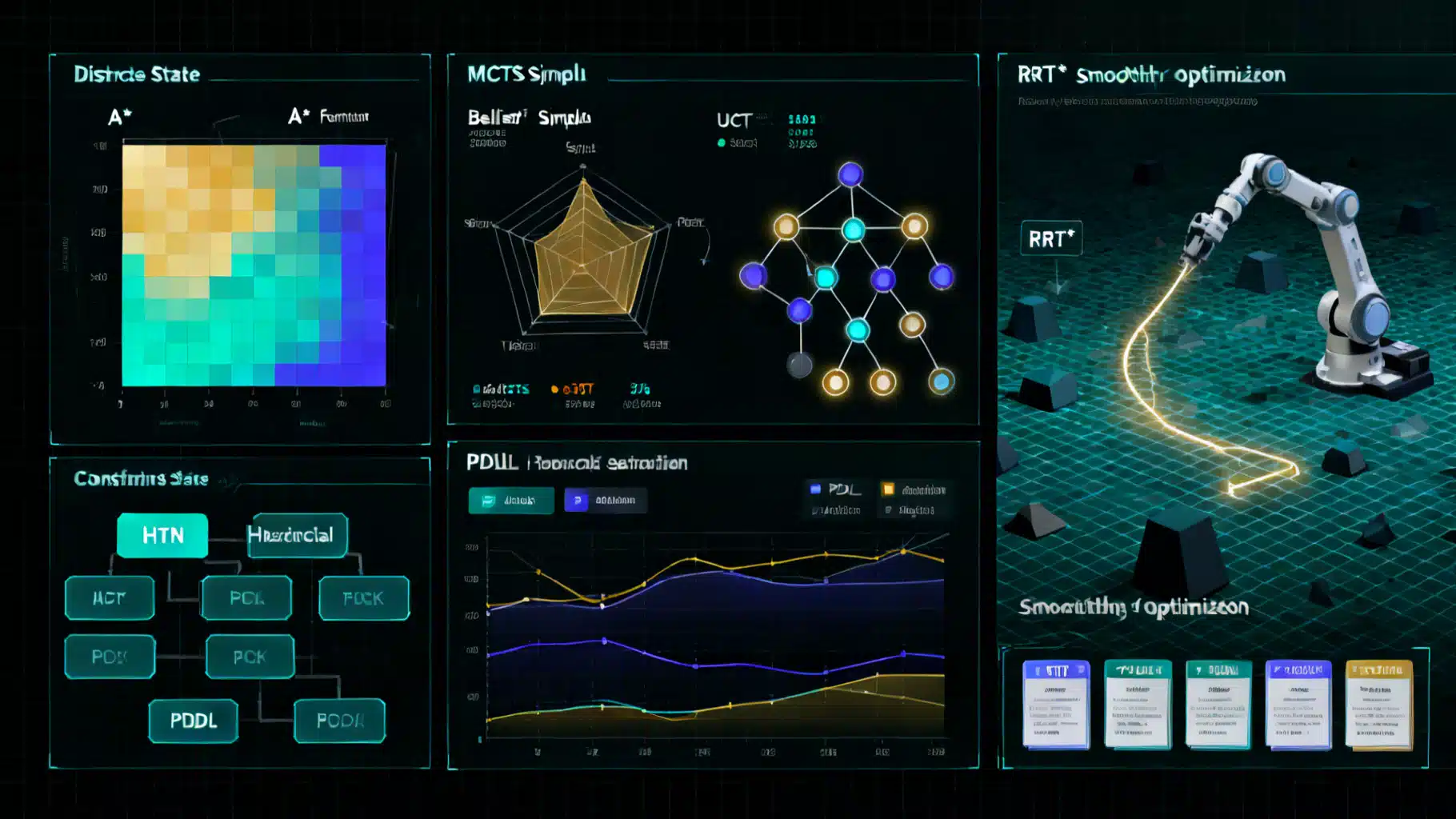
Image used for representation purposes only.
Overview
Planning is the quiet engine behind capable AI agents. It turns goals into sequences of actions that respect dynamics, constraints, and uncertainty. This article compares the main families of planning algorithms—classical symbolic planners, stochastic decision-theoretic methods, sampling-based planners for continuous spaces, tree search, and emerging LLM-driven planners—and gives a practical playbook for choosing and combining them.
The planning landscape at a glance
- Deterministic, discrete state/action models: heuristic state-space search (e.g., A*), partial-order planning, GraphPlan/SATPlan, hierarchical task networks (HTN), constraint- and optimization-based planning.
- Stochastic or partially observable settings: Markov decision processes (MDPs), POMDP planners, Monte Carlo Tree Search (MCTS) for online planning.
- Continuous state/control (robotics): sampling-based motion planning (PRM, RRT/RRT*), trajectory optimization, and MPC-style replanning.
- Learning-integrated: Dyna-style model-based RL, MCTS + learned models/heuristics, policy improvement via rollouts.
- LLM-native agents: plan-as-program prompting, ReAct-style reasoning + acting, Tree-of-Thought/Graph-of-Thought searches, planner–critic loops, tool-augmented planning with DSLs and verifiers.
Each family trades off modeling burden, performance guarantees, scalability, interpretability, and runtime responsiveness.
Classical symbolic planning
Symbolic planners assume a discrete world described by states, actions with preconditions and effects, and goal conditions (PDDL/STRIPS).
Heuristic state-space search (A*)
- Idea: Search the state graph from an initial state to a goal using f(n) = g(n) + h(n). The heuristic h estimates remaining cost.
- Strengths: Optimal with admissible h; flexible; well-understood. Heuristics derived from relaxations (e.g., delete-relaxation) scale surprisingly well.
- Weaknesses: Performance hinges on heuristic accuracy; large branching factors/long horizons can explode search.
- Use when: Deterministic domains with crisp action models; you need verifiable, cost-minimizing plans.
Partial-Order Planning (POP)
- Idea: Build a plan as a set of actions with partial ordering constraints, resolving threats via causal links.
- Strengths: Produces flexible, parallelizable plans; interpretable.
- Weaknesses: Can struggle with combinatorics in large domains.
- Use when: Concurrency matters and you want human-auditable plans.
GraphPlan and SATPlan
- GraphPlan: Builds a planning graph with mutex relations to quickly detect inapplicability; can extract short plans.
- SATPlan/SMT: Encode planning as satisfiability or constraint solving at a given horizon.
- Strengths: Powerful for bounded-horizon problems; leverages mature SAT/SMT technology.
- Weaknesses: Sensitive to horizon growth; may require iterative deepening.
- Use when: You can bound horizons and want strong unsat certificates if no plan exists.
Hierarchical Task Networks (HTN)
- Idea: Decompose high-level tasks into subtasks via domain-specific methods until primitive actions remain.
- Strengths: Excellent scalability via abstraction; plans are explainable by construction.
- Weaknesses: Requires domain engineering of methods; completeness depends on coverage.
- Use when: You have expert knowledge and recurring structures (e.g., workflows, ops runbooks, games).
Constraint- and optimization-based planning
- Encode planning/scheduling as CSP/MILP/CP-SAT and solve with general-purpose optimizers.
- Strengths: Handles resources, temporal constraints, and optimization naturally; strong guarantees.
- Weaknesses: Modeling effort; non-linear dynamics require approximations.
- Use when: Resource/temporal constraints dominate (e.g., logistics, staff scheduling, cloud capacity planning).
Decision-theoretic planning
When dynamics or observations are uncertain, you need to reason about probabilities and expected returns.
MDP planners
- Value iteration/policy iteration: Dynamic programming over the full state space for discounted rewards.
- Heuristic/anytime variants: LAO*, RTDP, LRTDP focus computation on reachable regions.
- Strengths: Provable convergence/optimality under standard assumptions.
- Weaknesses: State explosion; requires known transition/reward models.
- Use when: You have a factored or compact model and need optimal/near-optimal stationary policies.
POMDP planners
- Partial observability modeled via belief states (distributions over states).
- Point-based methods (e.g., PBVI) and online solvers (e.g., POMCP-style particle search) approximate value on reachable beliefs.
- Strengths: Principled treatment of uncertainty and information-gathering actions.
- Weaknesses: Computationally intense; belief management is tricky.
- Use when: Sensing is noisy and information actions are key (dialog, search, diagnostics, exploratory robotics).
Monte Carlo Tree Search (MCTS)
- Idea: Grow a search tree by repeated simulations; balance exploration/exploitation via UCT.
- Strengths: Strong anytime behavior; pairs well with learned value/policy priors; no need for full model tabulation.
- Weaknesses: High simulation cost; requires a generative model or learned simulator; can be myopic without good rollouts.
- Use when: Online decision-making under uncertainty, long horizons, or continuous action discretizations.
Continuous-space and motion planning
For robotics and control, the state is continuous and constraints are geometric or dynamical.
Sampling-based planners
- PRM: Sample milestones and connect to build a roadmap; good for multi-query settings.
- RRT/RRT*: Rapidly expand a tree towards random samples; RRT* refines toward optimal paths asymptotically.
- Strengths: Scale to high-dimensional spaces; handle complex obstacles.
- Weaknesses: Noisy, sometimes brittle in narrow passages; dynamics/kinematics require specialized steering.
- Use when: Navigation/manipulation in complex geometry; combine with local controllers/MPC.
Trajectory optimization and MPC
- Optimize a trajectory against dynamics and costs (e.g., iLQR, CHOMP), replan in a receding horizon.
- Strengths: Smooth, dynamically feasible motions; reacts to changes.
- Weaknesses: Local minima; requires good initializations and differentiable models.
- Use when: Real-time control with model fidelity and frequent replanning.
Learning-integrated planners
- Dyna-style model-based RL: Learn a model and plan inside it for sample efficiency.
- MCTS + learned models (AlphaZero/MuZero-style): Use neural priors and value functions to guide search.
- Heuristic learning: Learn domain-specific heuristics to accelerate classical search.
- Strengths: Leverages data to scale planning; adapts to non-stationary tasks.
- Weaknesses: Training cost and brittleness; weaker guarantees.
- Use when: Models are incomplete but data is plentiful and you can validate empirically.
LLM-native planning for tool-using agents
Large language models enable program-like planning through structured prompting and tool use.
- ReAct-style: Interleave reasoning traces with actions/tool calls, enabling situational replanning.
- Tree/Graph-of-Thought: Explore multiple candidate reasoning paths as a search; select via scoring or self-consistency.
- Planner–critic/reflection loops: Generate a plan, critique against constraints, refine iteratively.
- DSL/Schema-constrained planning: Ask the LLM to emit plans in a typed schema or domain language (e.g., PDDL steps, JSON workflows), then verify/execute.
- Retrieval-augmented planning: Pull procedures and past experiences from a memory or knowledge base to seed plans.
Strengths: Low modeling overhead; fast iteration; human-readable plans. Weaknesses: Hallucinations; inconsistent adherence to constraints; weak optimality/guarantees. Use when tasks are open-ended, knowledge-heavy, or benefit from tool APIs and lightweight oversight. Mitigate with verifiers, simulators, and execution monitors.
Core algorithms in 20 lines (pseudocode)
A* search (deterministic planning)
function A_star(start, is_goal, actions, step_cost, heuristic):
    open = PriorityQueue()
    open.push((0, start))
    g = {start: 0}
    parent = {start: None}
    while not open.empty():
        _, s = open.pop()  # node with smallest f = g + h
        if is_goal(s):
            return reconstruct_path(parent, s)
        for a in actions(s):
            s2 = a.apply(s)
            ng = g[s] + step_cost(s, a, s2)
            if s2 not in g or ng < g[s2]:
                g[s2] = ng
                f = ng + heuristic(s2)
                open.push((f, s2))
                parent[s2] = (s, a)
    return None
Value iteration (MDP)
function value_iteration(S, A, P, R, gamma, eps):
    V = {s: 0 for s in S}
    while True:
        delta = 0
        for s in S:
            V_old = V[s]
            V[s] = max(sum(P(s,a,s2) * (R(s,a,s2) + gamma * V[s2]) for s2 in S) for a in A(s))
            delta = max(delta, abs(V[s] - V_old))
        if delta < eps * (1 - gamma) / gamma:
            break
    policy = {s: argmax(A(s), key=lambda a: sum(P(s,a,s2) * (R(s,a,s2) + gamma * V[s2]) for s2 in S)) for s in S}
    return policy, V
MCTS with UCT
function MCTS(root, simulate, time_budget):
    while time_remaining(time_budget):
        path = select(root)
        leaf = path[-1]
        value = rollout(leaf, simulate)
        backpropagate(path, value)
    return best_child(root, exploitation_only=True)

function select(node):
    path = [node]
    while node.fully_expanded() and not node.terminal():
        node = argmax(node.children, key=lambda c: c.Q/c.N + c_uct * sqrt(log(node.N+1)/(c.N+1)))
        path.append(node)
    return path
Choosing the right planner: a practical playbook
- Deterministic, well-modeled tasks with clear costs: use A* (or IDA*, weighted A* for anytime). If resources/temporal constraints dominate, consider CP-SAT/MILP.
- Complex workflows with reusable know-how: HTN or hierarchical decomposition; add local A* inside subtasks.
- Short-horizon or bounded-depth puzzles: SAT/SMT encodings or GraphPlan.
- Uncertain transitions but good models: MDP solvers (LAO*, RTDP for focus on reachable states) or MCTS when online lookahead is acceptable.
- Noisy sensing and information gathering: POMDP online planners (particle-based) for robust behavior.
- Robotics navigation/manipulation: RRT* or PRM for feasibility; trajectory optimization/MPC for smooth, dynamic feasibility; replan as the world changes.
- Knowledge-heavy automation or web-tool agents: LLM planning with schema-constrained outputs, verified by simulators/executors; integrate retrieval for procedures.
Comparison dimensions that matter in practice
- Environment assumptions
- Deterministic vs stochastic vs partially observable vs adversarial.
- Discrete vs continuous state/action.
- Guarantees
- Completeness: finds a plan if one exists; Admissible/optimal vs bounded-suboptimal; safety constraints satisfied by construction.
- Scalability
- Branching factor, heuristic quality, horizon length, state factorization, and function approximation.
- Runtime behavior
- Anytime (improves with time) vs batch; online replanning vs offline policy synthesis.
- Modeling burden and data needs
- Hand-crafted PDDL/HTN vs learned models/heuristics vs prompt-based schemas.
- Interpretability and verification
- Causal links/HTN methods and CP/MILP are highly auditable; MDP policies and LLM plans need extra tracing/validation.
- Cost and efficiency
- Compute, memory, token/latency budgets; inference-time vs training-time trade-offs.
- Safety and constraint adherence
- Hard constraints via SAT/CP/MILP; shielding and runtime monitors; counterexample-guided refinement for learned/LLM components.
Evaluation methodology for agents
- Bench design
- Use task suites that reflect your deployment: deterministic puzzles, stochastic gridworlds, noisy web environments, robotics sims.
- Metrics
- Success rate, plan cost/length/return, wall-clock latency, sample/model-call efficiency, constraint violations, recovery success, reproducibility.
- Ablations and traces
- Vary heuristic strength, search depth, rollout policy, prompt templates, and memory size. Log search trees, belief updates, constraint solver traces, and LLM rationales.
- Offline vs online
- Validate plans in simulators; measure online replanning stability under perturbations. Include catastrophic case tests and long-horizon drift.
Hybrid design patterns that work
- HTN + A*/CP: Use HTN for structure; solve leaf subtasks optimally with search or optimization.
- MCTS + learned priors: Warm-start with value/policy networks or retrieval of similar tasks.
- RRT* + trajectory optimization: Find feasible skeletons, then smooth and make them dynamically feasible.
- LLM planner + verifier/executor: Emit a typed plan; validate against schemas, simulate effects, and enforce precondition/effect checks before acting.
- Model-predictive replanning: Wrap any planner in a receding-horizon loop to handle non-stationarity.
Common failure modes and mitigations
- Search blowup in large spaces: strengthen heuristics, use landmarks/pattern databases, prune with constraints, or move up a hierarchy.
- Myopic online planning: increase rollout depth, add learned value functions, or incorporate optimism bonuses.
- Brittleness to model error: perform belief tracking, ensemble models, or plan with uncertainty penalties; verify plans in simulation.
- LLM hallucinations and schema drift: strict JSON/PDDL schemas, function calling, unit tests for plan steps, and automatic repair via critics.
- Constraint violations at execution time: shielded controllers, runtime monitors, and fallback safe policies.
Implementation notes and tooling
- Classical planners: leverage existing PDDL planners and libraries for heuristic search; many support domain-independent heuristics and temporal extensions.
- Optimization: CP-SAT and MILP solvers integrate cleanly with scheduling/resource problems and can be combined with search for logic-heavy parts.
- RL/MDP: use standard RL libraries for value iteration/actor-critic baselines; adapt to planning via model-based components.
- Motion planning: robotics libraries provide PRM/RRT and trajectory optimization with collision checking.
- LLM agents: build around structured outputs, tool APIs, and verifiers; maintain traces and seeds for reproducibility.
A decision checklist
- Do you have a precise, deterministic model? If yes, start with A* or CP/SAT depending on constraints.
- Are uncertainty and information-gathering central? Consider POMDP or online MCTS with belief tracking.
- Is geometry/dynamics the bottleneck? Use sampling-based planning + trajectory optimization/MPC.
- Do you have reusable domain knowledge? Encode an HTN and solve subtasks optimally.
- Is the task open-ended and tool-driven? Use an LLM planner with strict schemas and a verifier/executor.
- Need quick wins under time pressure? Prefer anytime planners (weighted A*, MCTS) and hierarchical decompositions.
Takeaways
- There is no single best planner. Match assumptions and constraints to algorithmic strengths.
- For reliability, combine planners with verification, monitoring, and, when needed, human oversight.
- Hybrids—hierarchies over optimal leaf solvers, MCTS over learned models, LLM plans checked by formal tools—often give the best of both worlds.
Further reading roadmap
- Start with heuristic search and HTN for symbolic domains.
- Study MDP/POMDP foundations for uncertainty.
- Explore sampling-based motion planning for robotics.
- Add learning for priors/heuristics and MCTS for online decisions.
- Layer LLM planning with schemas, retrieval, and verification for practical agent systems.
Related Posts

Marc Benioff’s big 2026 bet: Agents, a $50B buyback—and a $300M AI token tab
Marc Benioff doubles down on the agentic enterprise with a $50B buyback, Headless 360, and a projected $300M Anthropic token bill—amid investor skepticism.

‘Gone in 9 Seconds’: Inside the “Claude Deletes Database” Incident
An AI coding agent running Claude reportedly erased a startup’s live database and backups in 9 seconds—exposing brittle guardrails in modern DevOps.

From Prototype to Production: Deploying Autonomous AI Agents Safely and at Scale
A practical blueprint for deploying autonomous AI agents to production—architecture, safety, reliability, evals, cost control, and ops patterns.