The Transformer Architecture, Visually Explained: From Tokens to Attention Maps
A clear, visual walkthrough of Transformer architecture—from tokens and positions to multi-head attention, residuals, and FFNs.
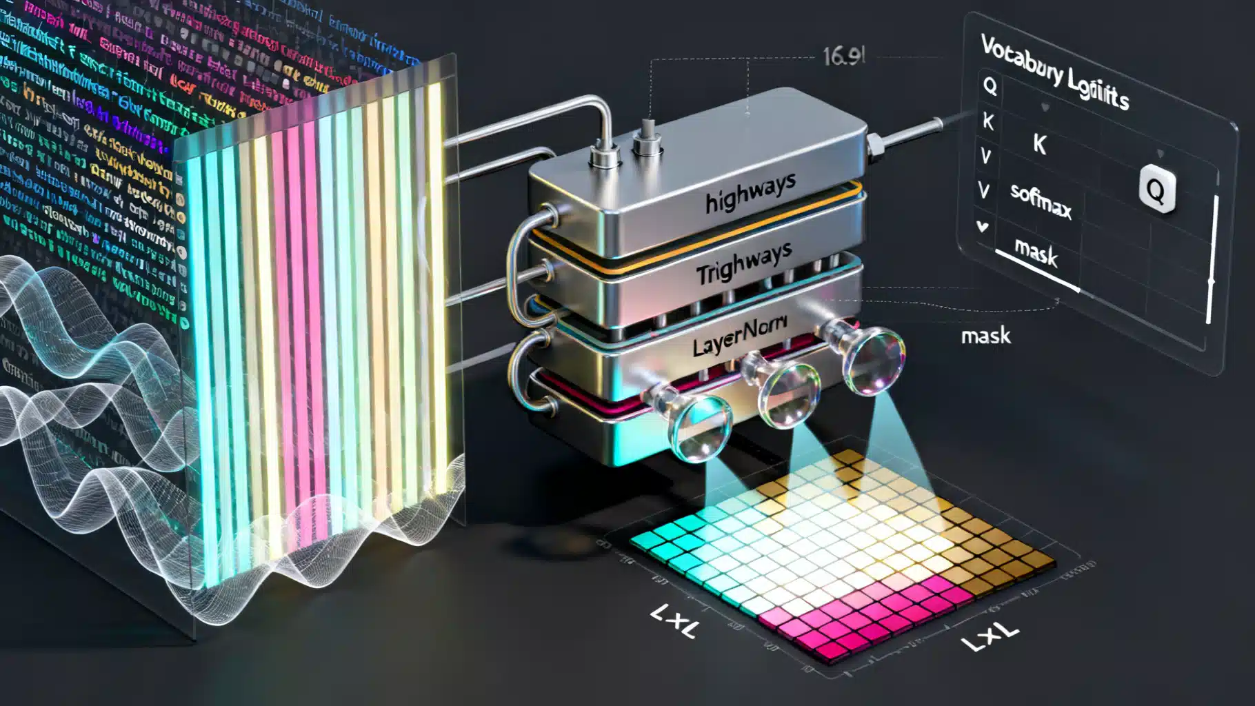
Image used for representation purposes only.
The Transformer Architecture, Visually Explained
Transformers power today’s language and vision models, yet the diagrams often feel dense: boxes labeled Q, K, V; arrows crisscrossing stacks; and heatmaps that look like abstract art. This article builds a visual, step‑by‑step mental model—from raw text to attention maps—so you can picture what each part is doing and why it works.
The 10,000‑Foot View
At a high level, a Transformer is a stack of identical blocks. Each block has two core parts: multi‑head self‑attention and a position‑wise feed‑forward network (FFN). Residual connections and layer normalization stabilize training.
A useful pipeline to visualize:
- Text → tokens → embeddings
- Add positional information
- Repeat N times: [Multi‑Head Self‑Attention → Add & Norm → Feed‑Forward → Add & Norm]
- Output head for the task (e.g., next‑token prediction)
[Text]
   ↓ tokenize
[Tokens] --lookup--> [Embeddings] + [Positional Info]
   ↓
┌ Transformer Block 1 ┐
│   Multi‑Head Attn   │
│  + Residual + Norm  │
│        FFN          │
│  + Residual + Norm  │
└─────────────────────┘
            ⋮ (repeat N times)
┌ Transformer Block N ┐
│   Multi‑Head Attn   │
│  + Residual + Norm  │
│        FFN          │
│  + Residual + Norm  │
└─────────────────────┘
   ↓
[Output logits] → [Predictions]
Step 1: Tokenization and Embeddings
- Tokenization splits text into subword units (e.g., “Trans”, “former”).
- Each token id indexes a learned vector from an embedding table E of size V × d_model, where V is the vocabulary size and d_model is the hidden width.
Shapes you can picture for a sequence length L:
- Tokens: L integers
- Embeddings: L × d_model (one row per token)
Tokens:     [ 314, 1027, 99,  7,  42 ]
             │     │     │  │   │
             └─┬───┴──┬──┘  │   │
               ▼      ▼     ▼   ▼
Embeddings: [e314, e1027, e99, e7, e42]  →  L × d_model matrix
Step 2: Positional Information
Self‑attention is permutation‑invariant; without position, the model can’t tell “cat chased dog” from “dog chased cat.” We inject order using:
- Sinusoidal encodings: fixed, smooth functions of position (helpful for extrapolation).
- Learned positional embeddings: a trainable table similar to token embeddings.
- Rotary/relative methods (e.g., RoPE, ALiBi): modify attention to encode distance directly.
Visually, imagine a position vector p_i added or fused to each token embedding e_i, yielding x_i = e_i + p_i (or a rotated variant). The result is still L × d_model.
Step 3: Multi‑Head Self‑Attention, One Picture at a Time
Attention lets each token “look at” other tokens to collect context. Each head projects inputs into queries (Q), keys (K), and values (V).
- Start with X (L × d_model)
- Linear projections produce:
- Q = XW_Q (L × d_k)
- K = XW_K (L × d_k)
- V = XW_V (L × d_v)
Scaled dot‑product attention per head:
- Scores = QKᵀ / √d_k → shape L × L
- Apply mask (e.g., causal mask for decoders to block future positions)
- Weights = softmax(Scores) → each row sums to 1
- Head output = Weights · V → shape L × d_v
Concatenate heads along the feature dimension (L × h·d_v), then project with W_O back to L × d_model.
Visual Walkthrough
Imagine 4 tokens: [“The”, “cat”, “chased”, “mice”]. After Q, K, V projections, a single head computes:
Q  : 4 × d_k
Kᵀ : d_k × 4
QKᵀ: 4 × 4  → attention scores (one row per query token)
softmax → attention weights (rows sum to 1)
weights · V → 4 × d_v (context‑aware features per token)
If you draw the 4×4 matrix as a heatmap, bright cells indicate strong attention. For the token “chased,” you might see attention peaks on “cat” (subject) and “mice” (object).
Why Multi‑Head?
One head might learn subject–verb links; another might track long‑range coreference; a third might focus on punctuation or syntax. Heads run in parallel on different subspaces (different W_Q, W_K, W_V), then merge. Visually: several heatmaps stacked side by side, each highlighting different patterns.
Head 1 heatmap: subject ↔ verb
Head 2 heatmap: object tracking
Head 3 heatmap: punctuation/phrase boundaries
...
Concatenate → Project → Rich, blended representation
Residual Connections and Layer Normalization
Two “highways” keep gradients stable and enable deep stacks:
- Add & Norm after attention: X + Dropout(Attn(X)) → LayerNorm
- Add & Norm after FFN: X + Dropout(FFN(X)) → LayerNorm
Architectures vary:
- Pre‑Norm: LayerNorm before attention/FFN sublayers (common in modern LLMs; trains more stably at scale)
- Post‑Norm: LayerNorm after the residual addition (original Transformer)
Visually, picture a main road (residual) running straight through the block, with side loops for attention and FFN that rejoin via addition.
The Feed‑Forward Network (FFN)
Each token’s vector passes through the same small MLP, position‑wise:
- FFN(x) = W_2 · σ(W_1 x + b_1) + b_2
- Typically expands to 4× the width, then projects back (e.g., d_ff ≈ 4·d_model)
- Activations: ReLU, GELU, or gated variants like SwiGLU
Shape intuition: L × d_model → L × d_ff → L × d_model. Visually, you can imagine every row (token) flowing through an identical two‑layer tower.
Encoder, Decoder, and Decoder‑Only (LLM) Stacks
- Encoder: self‑attention over the full input (no causal mask). Good for bidirectional understanding (e.g., BERT‑style tasks).
- Decoder: masked self‑attention (can’t peek at the future) plus cross‑attention to encoder outputs. Suited for sequence‑to‑sequence tasks (e.g., translation).
- Decoder‑only: a stack of masked self‑attention blocks without cross‑attention. This is the common LLM setup for next‑token prediction.
Visual cue: encoder attention heatmaps are symmetric in what they can reference; decoder self‑attention heatmaps are strictly lower‑triangular due to causal masking.
Training Objective and Inference Flow
- Objective: predict the next token given all previous tokens (causal LM). Cross‑entropy loss over the vocabulary.
- Teacher forcing during training: the model always sees the ground‑truth prefix.
- Inference: generate token by token, caching K and V to avoid recomputing attention over the whole prefix at each step.
Visual heuristic: imagine a sliding window that grows one token at a time, with KV “memory” blocks being stacked and reused.
Complexity and Long‑Context Considerations
- Vanilla attention is O(L²) in time and memory due to the L × L score matrix.
- Mitigations you might see in diagrams:
- Sparse/structured attention (blockwise, local, or global tokens)
- Low‑rank/linear attention approximations
- Efficient kernels (e.g., FlashAttention) that compute softmax attention with better memory locality
- Segmenting long sequences and using recurrence, memory tokens, or retrieval augmentation
When visualizing, replace the dense heatmap with banded or block‑sparse patterns.
Putting It Together: One Block, End‑to‑End
X_in (L × d_model)
  │
  ├─ LayerNorm (Pre‑Norm)
  │
  ├─ Multi‑Head Attention
  │    ├─ Q = XW_Q, K = XW_K, V = XW_V
  │    ├─ Scores = QKᵀ / √d_k
  │    ├─ + Mask (if causal)
  │    ├─ Weights = softmax(Scores)
  │    └─ AttnOut = Weights · V → concat heads → W_O
  │
  ├─ Residual Add: X_in + AttnOut
  │
  ├─ LayerNorm
  │
  ├─ Feed‑Forward Network (GELU / SwiGLU)
  │
  └─ Residual Add → X_out (L × d_model)
Stack N of these blocks. At the top, a linear layer ties or maps to vocabulary logits for language modeling.
How to Read and Create Useful Attention Visualizations
- Token–token heatmaps: rows are queries, columns are keys. Brightness shows how much one token attends to another.
- Head diversity: display multiple heads per layer; label notable patterns (e.g., “negation,” “quotation marks,” “subject link”).
- Layer depth: early layers often capture local syntax; deeper layers capture semantics and long‑range dependencies.
- Causal mask check: your heatmap should be strictly lower‑triangular in decoder‑only models.
- Sanity tests:
- Uniform attention early in training
- Sharp, interpretable heads after convergence
- For long inputs, verify that global or sentinel tokens receive attention as designed
Popular Variants You’ll Encounter (and How to Picture Them)
- Rotary Position Embeddings (RoPE): imagine rotating Q and K features by angle proportional to token index—attention becomes distance‑aware without extra tables.
- ALiBi: a bias added to attention scores that favors nearby tokens—visually a gradient overlay on the heatmap that dims far‑off positions.
- Gated FFNs (SwiGLU): two parallel projections, one gates the other—draw a valve controlling feature flow.
- Normalization tweaks: Pre‑Norm vs Post‑Norm; RMSNorm—same highway, just different rest stops.
- Parameter sharing: ALBERT‑style weight tying across layers—same block reused, drawn as a loop.
- Multimodal Transformers: add encoders for images/audio; cross‑attention connects modalities—picture parallel towers with bridges at multiple layers.
Memory and Throughput Intuition
- Attention memory scales with L² per head; KV caching at inference reduces recompute but not memory for the stored keys/values.
- Batch size and sequence length trade off. Visualize a rectangle where area ≈ memory; increase one side, the other must shrink unless you raise the budget.
- Mixed precision (FP16/BF16), tensor/sequence parallelism, and quantization compress the rectangles so you can fit more tokens or larger models.
Minimal Pseudocode to Anchor the Picture
# X: [L, d_model]
X = X + PositionalInfo(X)
for layer in range(N):
    # Pre‑Norm
    Y = LayerNorm(X)

    # Multi‑Head Self‑Attention
    Q = Y @ W_Q; K = Y @ W_K; V = Y @ W_V
    scores = (Q @ K.transpose(-1, -2)) / sqrt(d_k)
    scores = scores + mask  # e.g., causal: -inf above diagonal
    weights = softmax(scores, dim=-1)
    attn = (weights @ V) @ W_O

    X = X + attn  # residual

    # Feed‑Forward
    Z = LayerNorm(X)
    ff = W2 @ act(W1 @ Z + b1) + b2
    X = X + ff  # residual

logits = X @ E_T  # tie weights with embeddings (optional)
Picture each matrix op as a transformation of a tall, skinny block (the sequence) across its feature dimension, with attention temporarily expanding into an L × L sheet before collapsing back to L × d_v.
A Compact Mental Model
- Embeddings: give meaning to tokens
- Positional signals: give order to tokens
- Attention: mix information across tokens
- Multi‑head: mix in different “ways of looking”
- FFN: refine features per token
- Residual + Norm: keep learning stable
- Stacking: build depth → richer abstractions
Conclusion
Transformers are easier to grasp when you can picture the shapes: rows are tokens, columns are features, and attention is an L × L canvas that paints relationships. Once that canvas makes sense—queries, keys, values; masking; multi‑head composition—the rest of the architecture is just reliable plumbing: residuals, normalization, and per‑token MLPs. With this mental image, you can read any Transformer diagram, debug attention maps, and reason about variants with confidence.
Related Posts
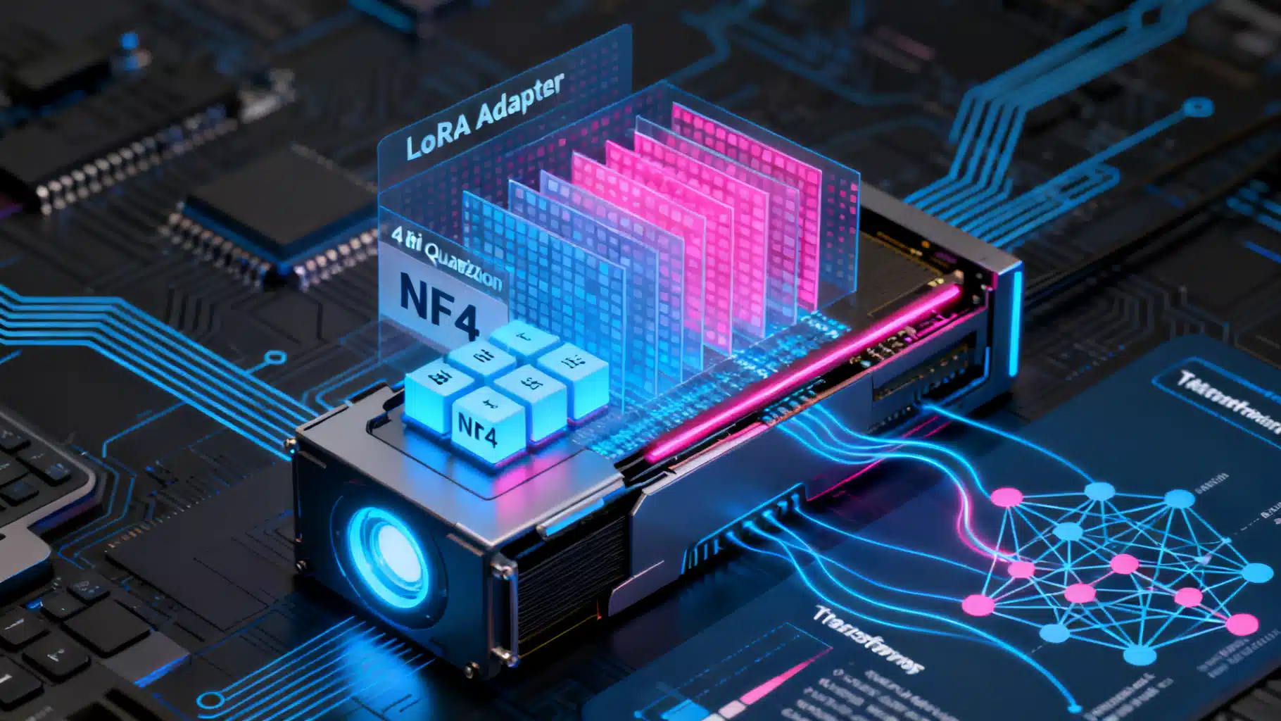
QLoRA Quantized Fine-Tuning: A Practical Guide to Training LLMs on a Single GPU
Step-by-step QLoRA guide with concepts, setup, memory tips, and code to fine-tune LLMs using 4-bit quantization on a single GPU.
API Consumer Analytics: From Raw Calls to Product Insight
A practical guide to API consumer analytics: what to track, how to instrument, and how to turn raw API calls into product and revenue insights.
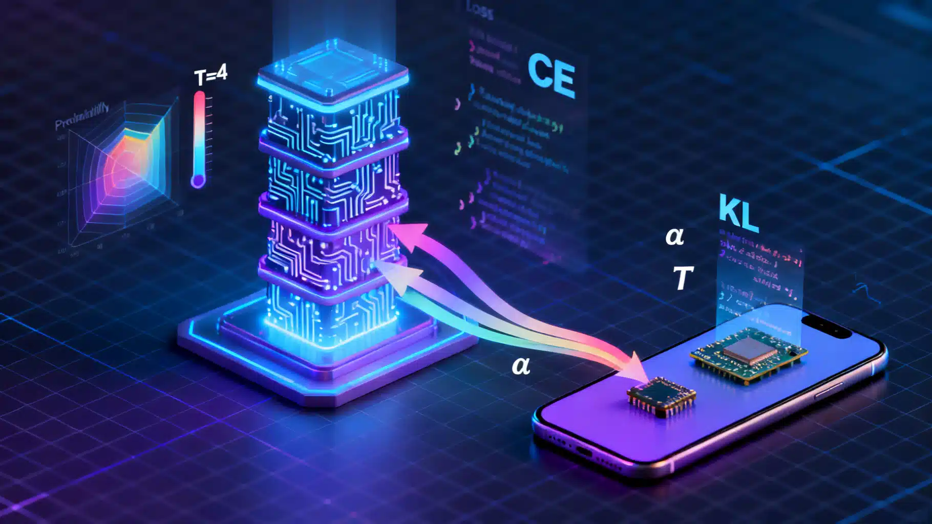
Knowledge Distillation Tutorial: Building Small, Fast Models that Perform
Hands-on knowledge distillation tutorial for compact models: concepts, PyTorch/Keras code, tuning tips, and deployment with quantization.