Diffusion Models for Image Generation: An Intuitive, Practical Guide
An intuitive, practical guide to diffusion models for image generation—how they work, architectures, guidance, sampling, and pro tips.

Image used for representation purposes only.
What Are Diffusion Models?
Diffusion models are a family of generative models that learn to create data by reversing a gradual noising process. During training, they learn how images become corrupted by noise step by step; at inference, they start from pure noise and progressively denoise to produce a coherent image. This approach has overtaken GANs in many image tasks thanks to its stability, scalability, and superior diversity.
At a high level:
- Forward (noising) process: repeatedly add Gaussian noise to an image until it becomes nearly pure noise.
- Reverse (denoising) process: learn a neural network that, given a noisy image and a time step t, predicts how to remove noise. Repeating this for T steps turns noise into an image.
The Core Idea, Intuitively
Imagine a Polaroid developing in reverse. Instead of details appearing over time, we begin with static and teach a model to remove just the right amount of noise at each step. If the removal is slightly off, the next steps can correct it—this iterative refinement is why diffusion models are so robust.
Training Objective: Denoising Score Matching
The goal is to learn the gradient of the log-density of data at different noise levels (the “score”). In practice, we train a network εθ(x_t, t, c) to predict the exact noise added to a clean image x₀ at time t, optionally conditioned on text or other inputs c.
Common parameterizations:
- Noise prediction (ε-prediction): predict the noise directly; simple and widely used.
- Data prediction (x₀-prediction): predict the clean image; can improve sharpness but may be less stable.
- v-prediction: a blend of ε and x₀ that often stabilizes training and improves sampling.
Loss functions are usually simple mean squared error between the true and predicted noise (or the chosen parameterization), sampled across random time steps.
The Noise Schedule
A schedule β₁…β_T controls how quickly noise is added in training and removed in sampling.
- Linear: simple baseline; works well.
- Cosine: smoother near endpoints; often improves quality.
- Karras/σ schedules: used in ODE/SDE samplers for better step allocation.
- VP/VE SDEs: continuous-time variants used by score-based diffusion; unify diffusion with stochastic calculus and enable advanced solvers.
Choosing a schedule affects both sample quality and the number of steps needed.
Architecture: Why U-Net Wins
The workhorse network is a U-Net with skip connections:
- Downsampling blocks capture global context.
- Upsampling blocks restore detail, fused via skip connections.
- Residual blocks + self-attention (at multiple resolutions) capture long-range dependencies and fine texture.
- Time embeddings (sinusoidal + MLP) inject the step t into every block.
For text-to-image, cross-attention layers fuse text features with image features. The text features come from a frozen language-image model (e.g., CLIP text encoder) or a large language model’s text encoder.
Conditioning and Guidance
Diffusion models are versatile because they accept conditions c:
- Text: prompts through a text encoder guide composition and style.
- Images: for image-to-image and inpainting you provide an initial image and/or a mask.
- Structural hints: ControlNets accept edges, pose, depth, or segmentation to steer layout.
Classifier-free guidance (CFG) is the most common way to strengthen conditioning without a separate classifier:
- Train with random “condition dropout” so the model learns both conditional and unconditional denoising.
- At inference, run the model twice (with and without the condition) and blend: x_guided = x_uncond + s · (x_cond − x_uncond).
- Guidance scale s controls prompt adherence vs. diversity; typical ranges are 3–9.
Sampling: From Hundreds of Steps to a Handful
Classical DDPM sampling uses ancestral stochastic steps and can take 50–1000 iterations. Modern samplers reduce this drastically:
- Deterministic samplers: DDIM, ODE-based methods (PNDM, DPM-Solver, Heun, Euler). These often reach good quality in 10–40 steps.
- Stochastic samplers: add controlled noise for diversity and can improve local detail.
- Karras-style schedulers: reparameterize noise levels (σ) for better step allocation.
Fewer steps mean faster inference, but going too low can cause washed-out details or prompt drift. For most modern latent diffusion models, 20–30 good steps are often sufficient.
Pixel-Space vs. Latent Diffusion
Early models operated directly on pixel space, which is computationally heavy. Latent diffusion compresses images with a Variational Autoencoder (VAE) into a smaller latent space (e.g., 4× downsampled with multiple channels). The diffusion model then operates on latents:
- Pros: massive speedups and memory savings; higher resolutions become feasible.
- Cons: VAE quality matters; a weak decoder can blur fine details or introduce artifacts.
Stable Diffusion popularized this approach by combining a powerful U-Net with a VAE and cross-attention text conditioning.
Inference Workflows You’ll Use in Practice
- Text-to-image: start from noise; denoise with text conditioning.
- Image-to-image: encode an input image to latents, add controlled noise (strength), then denoise with a prompt. Great for style transfer or edits.
- Inpainting/outpainting: use a mask to specify editable regions; only masked areas are resynthesized.
- Control-guided generation: pair prompts with edge maps, depth, pose, or sketches via ControlNet-like adapters.
Key knobs and their effects:
- Steps: 10–50 typical; more steps can improve detail but slow generation.
- CFG scale: higher enforces prompt, but too high causes oversaturation, repetition, or malformed anatomy.
- Sampler: Euler a/Heun are crisp and fast; DPM++ 2M/3M and DPM-Solver++ balance speed and fidelity; DDIM is deterministic and smooth.
- Seed: controls randomness; fix it for reproducibility.
- Resolution/aspect: larger sizes need more steps and VRAM; upscale with diffusion-based upscalers for best detail.
Minimal Pseudocode
Training loop (noise prediction variant):
for step in range(num_updates):
    x0, cond = sample_batch(dataset)            # images and optional text
    t = randint(1, T)                           # random time step
    eps = normal_like(x0)                       # Gaussian noise
    alpha_bar_t = cumprod(1 - beta) [t]         # schedule
    xt = sqrt(alpha_bar_t) * x0 + sqrt(1-alpha_bar_t) * eps

    if rand() < p_uncond:
        cond_in = None                           # condition dropout for CFG
    else:
        cond_in = cond

    eps_pred = model(xt, t, cond_in)             # U-Net forward
    loss = mse(eps_pred, eps)
    loss.backward(); optimizer.step()
Sampling (DDIM-style):
x = normal(shape)                                # start from noise
for t in reversed(range(1, T+1)):
    eps_cond = model(x, t, cond)
    eps_uncond = model(x, t, None)
    eps_hat = eps_uncond + cfg * (eps_cond - eps_uncond)

    x0_hat = predict_x0(x, t, eps_hat)           # parameterization-specific
    x = ddim_step(x, x0_hat, t, t-1, eta=0.0)    # or Euler/DPM-Solver, etc.
return decode_vae(x)
Extensions You’ll Encounter
- ControlNets: lightweight networks that condition on structure (edges, depth, pose), attached to the base U-Net via learned residuals.
- LoRA: low-rank adapters that fine-tune attention layers cheaply; ideal for style/persona injection with minimal VRAM.
- DreamBooth/Personalization: overfits a small set of subject images into the model or adapters; handle with care to avoid identity leakage.
- IP-Adapter and image conditioning: fuse image embeddings for consistent characters or styles.
- Distillation and consistency models: compress multi-step diffusion into few or single steps (e.g., LCM, consistency distillation, “turbo” variants) for real-time generation.
Strengths and Limitations
Strengths:
- Training stability: no adversarial min-max.
- Diversity and mode coverage: typically better than GANs.
- Fine control: via conditioning, guidance, and structure hints.
Limitations:
- Inference cost: multiple steps; mitigated by fast samplers or distilled models.
- VAE bottlenecks in latent diffusion: can blur microtexture; high-quality decoders help.
- Over-guidance artifacts: too-high CFG can cause oversharpening, banding, or repeated motifs.
- Data biases: models reflect their training data distributions; careful curation and safety filters are crucial.
Evaluating Image Quality
Common metrics and their caveats:
- FID/IS: correlate with perceived quality but can be gamed and are dataset-dependent.
- CLIP score: measures text-image alignment; high scores don’t always equal realism.
- Precision/Recall for generative models: tease apart fidelity vs. diversity.
In practice, combine automatic metrics with human evaluation and task-specific checks (e.g., brand safety, prompt compliance, artifact rates).
Practical Tips for Better Images
- Write precise prompts: subject, attributes, medium, style, lighting, composition, era, camera/lens, and mood.
- Use negative prompts for systematically unwanted features (e.g., “low-res, extra fingers, watermark”).
- Titrate CFG: start at 5–7; adjust if results are dull (raise) or overcooked (lower).
- Choose a sampler and schedule pair known to work well with your model; small step counts benefit more from modern ODE solvers.
- Upscale smartly: generate at a manageable size, then apply diffusion-based upscalers or specialized super-resolution models.
- For consistency across images: fix seeds and keep steps/sampler constant.
Safety, Legal, and Responsible Use
- Bias and fairness: inspect outputs across demographics and scenarios; adjust data, prompts, and filters to reduce harm.
- Safety filters: NSFW and content classifiers reduce risky outputs; pair them with prompt and output moderation.
- Attribution and IP: generated images may resemble training data styles or subjects; follow local laws, platform policies, and licensing requirements.
Where This Is Going
Research focuses on making diffusion faster and more controllable:
- Fewer-step sampling via improved solvers and distillation.
- Better conditioning with richer multimodal encoders and structured controls.
- Higher resolutions and photorealism via enhanced VAEs and attention efficiency (e.g., memory-optimized attention, tiling).
- Unified video and 3D generation using diffusion on sequences and fields.
Summary
Diffusion models generate images by learning to reverse a noise process. U-Net backbones with cross-attention, robust training via denoising objectives, and flexible conditioning make them state-of-the-art for creative and practical imaging. With the right sampler, schedule, and guidance scale, you can reliably turn prompts—or sketches and masks—into detailed, controllable visuals. As fast samplers and distilled models mature, diffusion is moving from batch generation to interactive, near-real-time creativity.
Related Posts
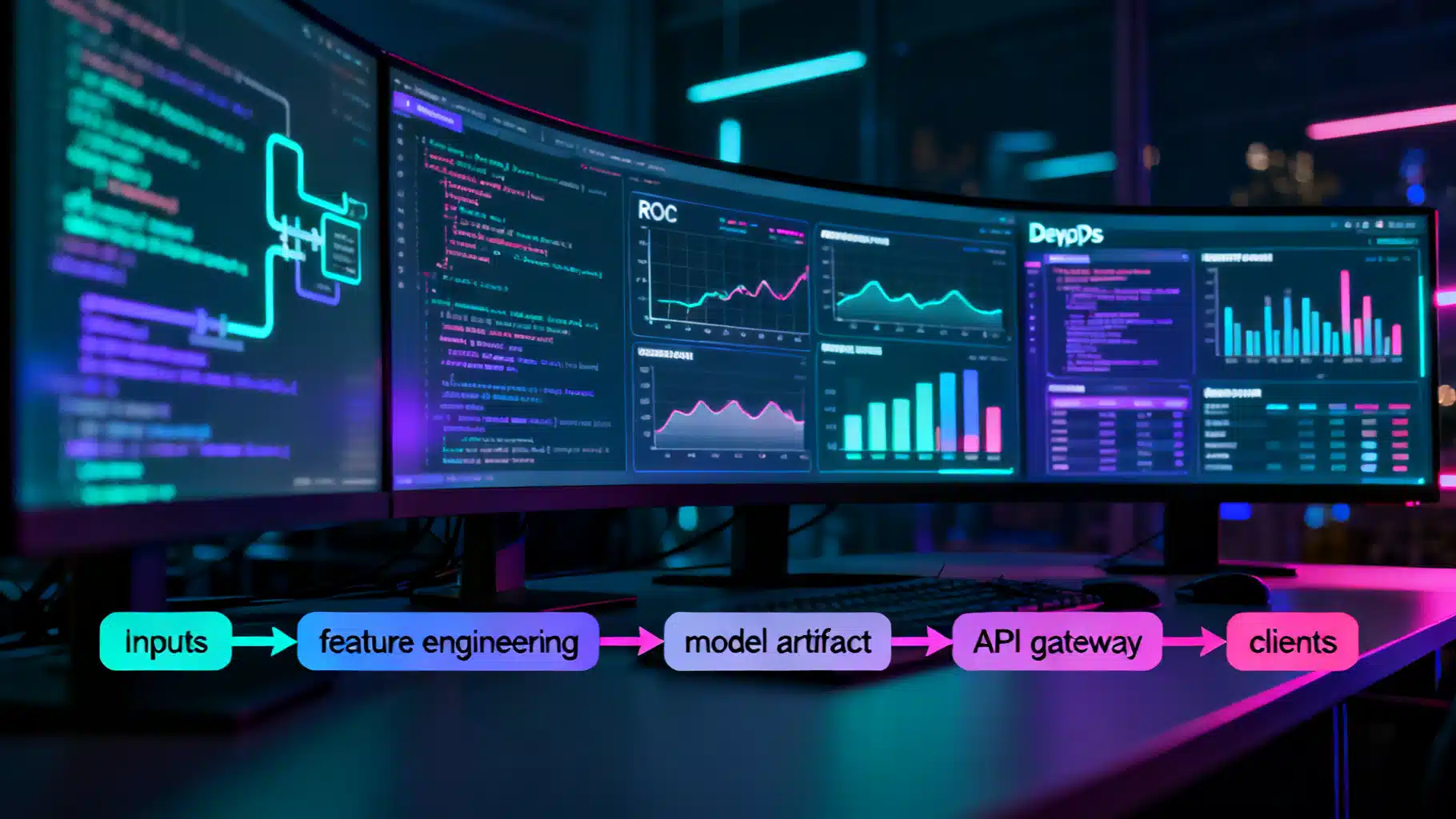
Build a Production‑Ready Predictive Analytics API: A Step‑by‑Step Tutorial
Build a production-ready predictive analytics API with Python and FastAPI—training, serving, security, testing, and MLOps in one tutorial.
From Dataset to Endpoint: A Practical AI Text Classification API Tutorial
Build, deploy, and scale a production-ready AI text classification API with Python and FastAPI—training, serving, security, metrics, and monitoring.
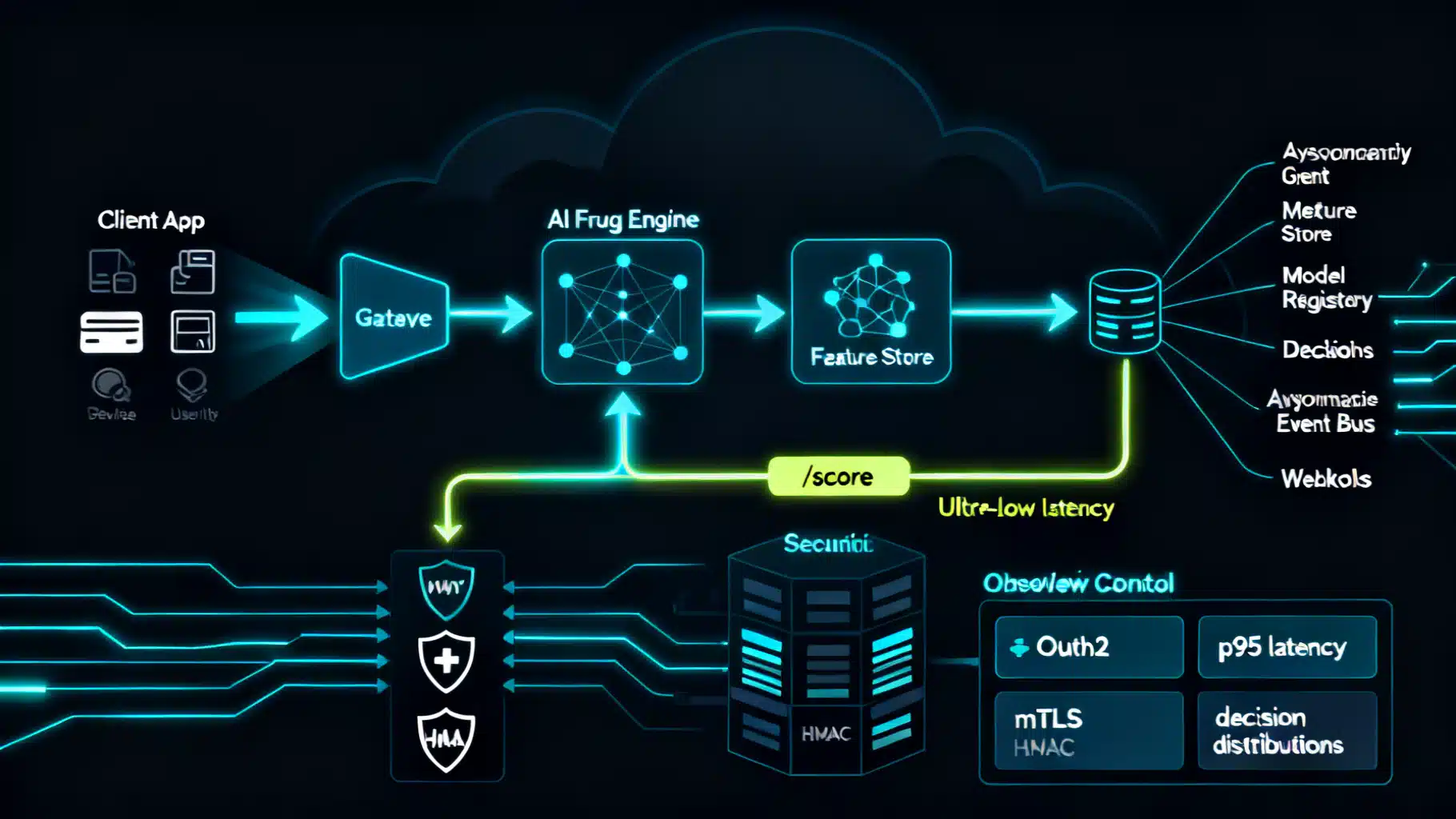
AI Fraud Detection API Integration: Architecture, Security, and Implementation Guide
Practical guide to AI fraud detection API integration: architecture, payloads, security, thresholds, MLOps, and operations with code samples.